The Fourier transform is an essential tool in many fields, be it in Physics, Signal Processing, or Mathematics. The method that is probably the most known to calculate it numerically is called the FFT for Fast Fourier Transform. In this little tutorial, I propose to try to understand and implement this algorithm in an efficient way. I will use the language Julia, but it should be possible to follow using other languages such as Python or C. We will compare the results obtained with those given by the Julia port of the FFTW library.

This tutorial is intended for people who have already had the opportunity to encounter the Fourier transform, but who have not yet implemented it. It is largely based on the third edition of Numerical Recipes^[1], which I encourage you to consult: it is a gold mine.

Table of contents

Some reminders on the discrete Fourier transform

The discrete Fourier transform is a transformation that follows from the Fourier transform and is, as its name indicates, adapted for discrete signals. In this first part I propose to discover how to build the discrete Fourier transform and then understand why the fast Fourier transform is useful.

The Fourier transform

This tutorial is not intended to present the Fourier transform. However, there are several definitions of the Fourier transform and even within a single domain, several are sometimes used. We will use the following: for a function $f$, its Fourier transform $\hat{f}$ is defined by:

From the Fourier transform to the discrete Fourier transform

As defined in the previous section, the Fourier transform of a signal is a continuous function of the variable $\nu$. However, to represent any signal, we can only use a finite number of values. To do this we proceed in four steps:

1. We sample (or discretize) the signal to analyze. This means that instead of working on the function that associates the value of the signal with the variable $x$, we will work on a discrete series of values of the signal. In the case of the FFT, we sample with a constant step. For example if we look at a temporal signal like the value of a voltage read on a voltmeter, we could record the value at each tic of a watch.

2. We window the discretized signal. This means that we keep only a finite number of points of the signal.

3. We sample the Fourier transform of the signal to obtain the discrete Fourier transform.

4. We window the discrete Fourier transform for storage.

I suggest you to reason on a toy signal which will have the shape of a Gaussian. This makes the reasoning a little simpler because the Fourier transform of a real Gaussian is also a real Gaussian^[2], which simplifies the graphical representations.

More formally, we have:

Let's first look at the sampling. Mathematically, we can represent the process by the multiplication of the signal $f$ by a Dirac comb of period $T$, $ш_T$. The Dirac comb is defined as follows:

With $\delta$ the Dirac distribution. Here is the plot that we can obtain if we represent $f$ and $g=ш_T\times f$ together:

The Fourier transform of the new $g$ function is written ^[3] :

If we put $f[k]=f(kT)$ the sampled signal and $\nu_{text{ech}} = \frac{1}{T}$ the sampling frequency, we have:

If we plot the Fourier transform of the starting signal $\hat{f}$ and that of the sampled signal $\hat{g}$, we obtain the following plot:

Information

We notice that the sampling of the signal has led to the periodization of its Fourier transform. This leads to an important property in signal processing: the Nyquist-Shanon criterion, and one of its consequences, spectrum aliasing. I let you consult the Wikipedia article about this if you are interested, but you can have a quick idea of what happens if you draw the previous plot with a too large sampling: the bells of the sampled signal transform overlap.

We can then look at the windowing process. There are several methods that each have their advantages, but we will focus here only on the rectangular window. The principle is simple: we only look at the values of $f$ for $x$ between $-x_0$ and $+x_0$. This means that we multiply the function $f$ by a gate function $\Pi_{x_0}$ which verifies:

Graphically, here is how we could represent $h$ and $f$ together.

Concretely, this is equivalent to limiting the sum of the Dirac comb to a finite number of terms. We can then write the Fourier transform of $h=Pi_{x_0} \times ш_T \times f$ :

We can now proceed to the last step: sampling the Fourier transform. Indeed, we can only store a finite number of values on our computer and, as defined, the function $\hat{h}$ is continuous. We already know that it is periodic, with period $\nu_{\text{ech}}$, so we can store only the values between $0$ and $\nu_{\text{ech}}$. We still have to sample it, and in particular to find the adequate sampling step. It is clear that we want the sampling to be as "fine" as possible, in order not to miss any detail of the Fourier transform! For this we can take inspiration from what happened when we sampled $f$: its Fourier transform became periodic, with period $\nu_{\text{ech}}$. Now the inverse Fourier transform (the operation that allows to recover the signal from its Fourier transform) has similar properties to the Fourier transform. This means that if we sample $\hat{h}$ with a sampling step $\nu_s$, then its inverse Fourier transform becomes periodic with period $1/\nu_s$. This gives a low limit on the values that $\nu_s$ can take ! Indeed, if the inverse transform has a period smaller than the width of the window ($1/\nu_s < 2x_0$), then the reconstructed signal taken between $-x_0$ and $x_0$ will not correspond to the initial signal $f$ !

So we choose $\nu_s = \frac{1}{2x_0}$ to discretize $\hat{h}$. We use the same process of multiplication by a Dirac comb to discretize. In this way we obtain the Fourier transform of a new function $l$ :

This notation is a bit complicated, and we can be more interested in $\hat{l}[n]=\hat{l}(n\nu_s)$ :

To get the last line, I re-indexed $f[k]$ to start at 0, noting $N$ the number of samples. I then assumed that the window size corresponded to an integer number of samples, i.e. that $2x_0 = N\times T$, which is rewritten as $N\times \nu_s = \nu_{\text{ech}}$. This expression is the discrete Fourier transform of the signal.

This problem is solved quite simply by windowing the discrete Fourier transform. Since the transform has been periodized by the sampling of the starting signal, it is enough to store one period of the transform to store all the information contained in it. The choice which is generally made is to keep all the points between O and $\nu_{\text{ech}}$. This allows to use only positive $n$, and one can easily reconstruct the plot of the transform if needed by inverting the first and the second half of the computed transform. In practice (for the implementation), the discrete Fourier transform is thus given by :

To conclude on our example function, we obtain the following plot:

Calculating the discrete Fourier transform

So we have at our disposal the expression of the discrete Fourier transform of a signal $f$:

This s the expression of a matrix product which would look like this:

with

Those in the know will notice that this is a Vandermonde matrix on the roots of the unit.

So this calculation can be implemented relatively easily!

function naive_dft(x)
  N = length(x)
  k = reshape(0:(N-1), 1, :)
  n = 0:(N-1)
  M = @. exp(-2im * π * k * n / N)
  M * x
end

And to check that it does indeed give the right result, it is enough to compare it with a reference implementation:

using FFTW

a = rand(1024)
b = fft(a)
c = naive_dft(a)
b ≈ c

The last block evaluates to true, which confirms that we are not totally off the mark!

However, is this code effective? We can check by comparing the memory footprint and execution speed.

using BenchmarkTools

@benchmark fft(a) setup=(a = rand(1024))

LoadError: UndefVarError: `@benchmark` not defined
in expression starting at none:1

@benchmark naive_dft(a) setup=(a = rand(1024))

LoadError: UndefVarError: `@benchmark` not defined
in expression starting at none:1

So our implementation is really slow (about 10,000 times) and has a very high memory footprint (about 500 times) compared to the benchmark implementation! To improve this, we will implement the fast Fourier transform.

Why a fast Fourier transform algorithm?

Before getting our hands dirty again, let's first ask the question: is it really necessary to try to improve this algorithm?

Before answering directly, let us look at some applications of the Fourier transform and the discrete Fourier transform.

The Fourier transform has first of all a lot of theoretical applications, whether it is to solve differential equations, in signal processing or in quantum physics. It also has practical applications in optics and in spectroscopy.

The discrete Fourier transform also has many applications, in signal analysis, for data compression, multiplication of polynomials or the computation of convolution products.

Our naive implementation of the discrete Fourier transform has a time and memory complexity in $\mathcal{O}(N^2)$ with $N$ the size of the input sample, this is due to the storage of the matrix and the computation time of the matrix product. Concretely, if one wished to analyze a sound signal of 3 seconds sampled at 44kHz with data stored on simple precision floats (4 bytes), it would thus be necessary approximately $2\times(44000\times3)^2\times 4\approx100\;000\;000\;000$ bytes of memory (a complex number is stored on 2 floats) We can also estimate the time necessary to make this calculation. The median time for 1024 points was 38.367 ms. For our 3 seconds signal, it would take about $38.867\times\left(\frac{44000\times3}{1024}\right)^2\approx 637\;537$ milliseconds, that is more than 10 minutes !

One can easily understand the interest to reduce the complexity of the calculation. In particular the fast Fourier transform algorithm (used by the reference implementation) has a complexity in $\mathcal{O}(N\log N)$. According to our benchmark, the algorithm processes a 1024-point input in 23.785µs. It should therefore process the sound signal in about $23.785\times\frac{44000\times\log(44000\times3)}{1024\times\log1024}\approx 5\;215$ microseconds, that is to say about 120000 times faster than our algorithm. We can really say that the fast of Fast Fourier Transform is not stolen !

We saw how the discrete Fourier transform was constructed, and then we naively tried to implement it. While this implementation is relatively simple to implement (especially with a language like Julia that facilitates matrix manipulations), we also saw its limitations in terms of execution time and memory footprint.

It's time to move on to the FFT itself!

Implementing the FFT

In this part we will implement the FFT by starting with a simple approach, and then making it more complex as we go along to try to calculate the Fourier transform of a real signal in the most efficient way possible. To compare the performances of our implementations, we will continue to compare with the FFTW implementation.

My first FFT

We have previously found the expression of the discrete Fourier transform :

The trick at the heart of the FFT algorithm is to notice that if we try to cut this sum in two, separating the even and odd terms, we get (assuming $N$ is even), for $n < N/2$ :

where $\hat{f}^\text{even}$ and $\hat{f}^\text{odd}$ are the Fourier transforms of the sequence of even terms of $f$ and of the sequence of odd terms of $f$. We can therefore compute the first half of the Fourier transform of $f$ by computing the Fourier transforms of these two sequences of length $N/2$ and recombining them. Similarly, if we compute $\hat{f}[n+N/2]$ we have :

This means that by computing two Fourier transforms of length $N/2$, we are able to compute two elements of a Fourier transform of length $N$. Assuming for simplicity that $N$ is a power of two^[4], this naturally draws a recursive implementation of the FFT. According to the master theorem, this algorithm will have complexity $\mathcal{O}(N\log_2 N)$, which is much better than the first naive algorithm we implemented, which has complexity in $\mathcal{O}(N^2)$.

function my_fft(x)
  # Stop condition, the TF of an array of size 1 is this same array.
  if length(x) <= 1
    x
  else
    N = length(x)
    # Xᵒ contains the TF of odd terms and Xᵉ that of even terms.
    # The subtlety being that Julia's tablals start at 1 and not 0.
    Xᵒ = my_fft(x[2:2:end])
    Xᵉ = my_fft(x[1:2:end])
    factors = @. exp(-2im * π * (0:(N/2 - 1)) / N)
    [Xᵉ .+ factors .* Xᵒ; Xᵉ .- factors .* Xᵒ]
  end
end

We can check as before that code gives a fair result, then compare its runtime qualities with the reference implementation.

@benchmark fft(a) setup=(a = rand(1024))

LoadError: UndefVarError: `@benchmark` not defined
in expression starting at none:1

@benchmark my_fft(a) setup=(a = rand(1024))

LoadError: UndefVarError: `@benchmark` not defined
in expression starting at none:1

We can see that we have improved the execution time (by a factor of 8) and the memory footprint of the algorithm (by a factor of 13), without getting closer to the reference implementation.

Analysis of the first implementation

Let's go back to the previous code:

function my_fft(x)
  # Stop condition, the TF of an array of size 1 is this same array.
  if length(x) <= 1
    x
  else
    N = length(x)
    # Xᵒ contains the TF of odd terms and Xᵉ that of even terms.
    # The subtlety being that Julia's tablals start at 1 and not 0.
    Xᵒ = my_fft(x[2:2:end])
    Xᵉ = my_fft(x[1:2:end])
    factors = @. exp(-2im * π * (0:(N/2 - 1)) / N)
    [Xᵉ .+ factors .* Xᵒ; Xᵉ .- factors .* Xᵒ]
  end
end

And let's try to keep track of the memory allocations. For simplicity, we can assume that we are working on an array of 4 elements, [f[0], f[1], f[2], f[3]]. The first call to my_fft keeps in memory the initial array, then launches the fft on two sub-arrays of size 2: [f[0], f[2]] and [f[1], f[3]], then recursive calls keep in memory before recombining the arrays [f[0]] and [f[2]] then [f[1]] and [f[3]]. At most, we have $log_2(N)$ arrays allocated with sizes divided by two each time. Not only do these arrays take up memory, but we also waste time allocating them!

However, if we observe the definition of the recurrence we use, at each step $i$ (i.e. for each array size, $N/2^i$), the sum of the intermediate array sizes is always $N$. In other words, this gives the idea that we could save all these array allocations and use the same array all the time, provided that we make all the associations of arrays of the same size at the same step.

Schematically we can represent the FFT process for an array with 8 elements as follows:

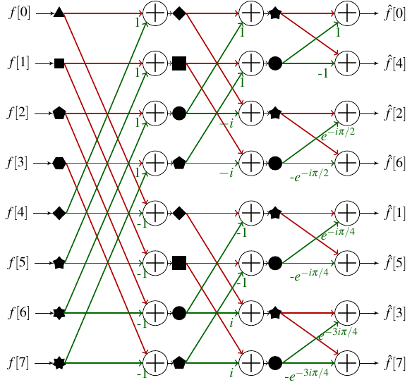
How to read this diagram? Each column corresponds to a depth of the recurrence of our first FFT. The leftmost column corresponds to the deepest recurrence: we have cut the input array enough to arrive at subarrays of size 1. These 8 sub-tables are symbolized by 8 different geometrical shapes. We then go to the next level of recurrence. Each pair of sub-tables of size 1 must be combined to create a sub-table of size 2, which will be stored in the same memory cells as the two sub-tables of size 1. For example, we combine the subarray ▲ that contains $f[0]$ and the subarray ◆ that contains $f[4]$ using the formula demonstrated earlier to form the array $[f[0] + f[4], f[0] - f[4]]$, which I call in the following ◆, and store the two values in position 0 and 4. The colors of the arrows allow us to distinguish those bearing a coefficient (which correspond to the treatment we give to the subarray $\hat{f}^{\text{odd}}$ in the formulas of the previous section). After having constructed the 4 sub-tables of size 2, we can proceed to a new step of the recurrence to compute two sub-tables of size 4. Finally the last step of the recurrence combines the two subarrays of size 4 to compute the array of size 8 which contains the Fourier transform.

Based on this scheme we can think of having a function whose main loop would calculate successively each column to arrive at the final result. In this way, all the calculations are performed on the same array and the number of allocations is minimized! There is however a problem: we see that the $\hat{f}[k]$ do not seem to be ordered at the end of the process.

In reality, these $\hat{f}[k]$ are ordered via a reverse bit permutation. This means that if we write the indices $k$ in binary, then reverse this writing (the MSB becoming the LSB^[5]), we obtain the index at which $\hat{f}[k]$ is found after the FFT algorithm. The permutation process is described by the following table in the case of a calculation on 8 elements.

If we know how to calculate the reverse permutation of the bits, we can simply reorder the array at the end of the process to obtain the right result. However, before jumping on the implementation, it is interesting to look at what happens if instead we reorder the input array via this permutation.

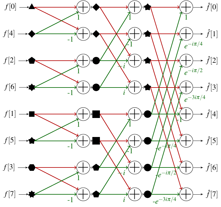
We can see that by proceeding in this way we have a simple ordering of the sub-tables. Since in any case it will be necessary to proceed to a permutation of the table, it is interesting to do it before the calculation of the FFT.

Calculate the reverse permutation of the bits

We must therefore begin by being able to calculate the permutation. It is possible to perform the permutation in place simply once we know which elements to exchange. Several methods exist to perform the permutation, and a search in Google Scholar will give you an overview of the wealth of approaches.

We can use a little trick here: since we are dealing only with arrays whose size is a power of 2, we can write the size $N$ as $N=2^p$. This means that the indices can be stored on $p$ bits. We can then simply calculate the permuted index via binary operations. For example if $p=10$ then the index $797$ could be represented as: 1100011101.

We can separate the inversion process in several steps. First we exchange the 5 most significant bits and the 5 least significant bits. Then on each of the half-words we invert the two most significant bits and the two least significant bits (the central bits do not change). Finally on the two bits words that we have just exchanged, we exchange the most significant bit and the least significant bit.

An example of implementation would be the following:

bit_reverse(::Val{10}, num) = begin
  num = ((num&0x3e0)>>5)|((num&0x01f)<<5)
  num = ((num&0x318)>>3)|(num&0x084)|((num&0x063)<<3)
  ((num&0x252)>>1)|(num&0x084)|((num&0x129)<<1)
end

An equivalent algorithm can be applied for all values of $p$, you just have to be careful not to change the central bits anymore when you have an odd number of bits in a half word. In the following there is an example for several word lengths.

bit_reverse(::Val{64}, num) = bit_reverse(Val(32), (num&0xffffffff00000000)>>32)|(bit_reverse(Val(32), num&0x00000000ffffff)<<32)
bit_reverse(::Val{32}, num) = bit_reverse(Val(16), (num&0xffff0000)>>16)|(bit_reverse(Val(16), num&0x0000ffff)<<16)
bit_reverse(::Val{16}, num) = bit_reverse(Val(8), (num&0xff00)>>8)|(bit_reverse(Val(8), num&0x00ff)<<8)
bit_reverse(::Val{8}, num) = bit_reverse(Val(4), (num&0xf0)>>4)|(bit_reverse(Val(4), num&0x0f)<<4)
bit_reverse(::Val{4}, num) =bit_reverse(Val(2), (num&0xc)>>2)|(bit_reverse(Val(2), num&0x3)<<2)
bit_reverse(::Val{3}, num) = ((num&0x1)<<2)|((num&0x4)>>2)|(num&0x2)
bit_reverse(::Val{2}, num) = ((num&0x2)>>1 )|((num&0x1)<<1)
bit_reverse(::Val{1}, num) = num

Then we can do the permutation itself. The algorithm is relatively simple: just iterate over the array, calculate the inverted index of the current index and perform the inversion. The only subtlety is that the inversion must be performed only once per index of the array, so we discriminate by performing the inversion only if the current index is lower than the inverted index.

function reverse_bit_order!(X, order)
  N = length(X)
  for i in 0:(N-1)
    j = bit_reverse(order, i)
    if i<j
      X[i+1],X[j+1]=X[j+1],X[i+1]
    end
  end
  X
end

My second FFT

We are now sufficiently equipped to start a second implementation of the FFT. The first step will be to compute the reverse bit permutation. Then we will be able to compute the Fourier transform following the scheme shown previously. To do this we will store the size $n_1$ of the sub-arrays and the number of cells $n_2$ in the global array that separate two elements of the same index in the sub-arrays. The implementation can be done as follows:

function my_fft_2(x)
  N = length(x)
  order = Int(log2(N))
  @inbounds reverse_bit_order!(x, Val(order))
  n₁ = 0
  n₂ = 1
  for i=1:order # i done the number of the column we are in.
    n₁ = n₂ # n₁ = 2ⁱ-¹
    n₂ *= 2 # n₂ = 2ⁱ
    
    step_angle = -2π/n₂
    angle = 0
    for j=1:n₁ # j is the index in Xᵉ and Xᵒ
      factors = exp(im*angle) # z = exp(-2im*π*(j-1)/n₂)
      angle += step_angle # a = -2π*(j+1)/n₂
      
      # We combine the element j of each group of subarrays
      for k=j:n₂:N
        @inbounds x[k], x[k+n₁] = x[k] + factors * x[k+n₁], x[k] - factors * x[k+n₁]
      end
    end
  end
  x  
end

We can again measure the performance of this implementation. To keep the comparison fair, the fft! function should be used instead of fft, as it works in place.

@benchmark fft!(a) setup=(a = rand(1024) |> complex)

LoadError: UndefVarError: `@benchmark` not defined
in expression starting at none:1

@benchmark my_fft_2(a) setup=(a = rand(1024) .|> complex)

LoadError: UndefVarError: `@benchmark` not defined
in expression starting at none:1

We have significantly improved our execution time and memory footprint. We can see that there are zero bytes allocated (this means that the compiler does not need to store the few intermediate variables in RAM), and that the execution time is close to that of the reference implementation.

The special case of a real signal

So far we have reasoned about complex signals, which use two floats for storage. However in many situations we work with real value signals. Now in the case of a real signal, we know that $\hat{f}$ verifies $\hat{f}(-\nu) = \overline{\hat{f}(\nu)}$. This means that half of the values we calculate are redundant. Although we calculate the Fourier transform of a real signal, the result can be a complex number. In order to save storage space, we can think of using this half of the array to store complex numbers. For this, two properties will help us.

Property 1: Compute the Fourier transform of two real functions at the same time

If we have two real signals $f$ and $g$, we can define the complex signal $h=f+ig$. We then have:

We can notice that

Combining the two we have

Property 2 : Compute the Fourier transform of a single function

The idea is to use the previous property by using the signal of the even and the odd elements. In other words for $k=0...N/2-1$ we have $h[k]=f[2k]+if[2k+1]$.

Then we have:

We can recombine the two partial transforms. For $k=0...N/2-1$ :

Using the first property, we then have:

Calculation in place

The array $h$, which is presented previously, is complex-valued. However the input signal is real-valued and twice as long. The trick is to use two cells of the initial array to store a complex element of $h$. It is useful to do the calculations with complex numbers before starting to write code. For the core of the FFT, if we note $x_i$ the array at step $i$ of the main loop, we have:

With the organization we choose, we can replace $\text{Re}(x[k])$ with $x[2k]$ and $\text{Im}(x[k])$ with $x[2k+1]$. We also note that we can replace $\text{Re}(x[k+n_1])$ with $x[2(k+n_1)]$ or even better $x[2k+n_2]$.

The last step is the recombination of $h$ to find the final result. The formula in property 2 is rewritten after an unpleasant but uncomplicated calculation:

There is a particular case where this formula does not work: when $k=0$ we leave the array $h$ which contains only $N/2$ elements. However we can use the symmetry of the Fourier Transform to see that $h[N/2]=h[0]$. The case $k=0$ then simplifies enormously:

To perform the calculation in place, it is useful to be able to calculate $\hat{x}[N/2-k]$ at the same time that we calculate $\hat{x}[k]$. Reusing the previous results and the fact that $e^{-2i\pi(N/2-k)/N}=-e^{2i\pi k/N}$, we find:

After this little unpleasant moment, we are ready to implement a new version of the FFT!

An FFT for the reals

Since the actual computation of the FFT is done on an array that is half the size of the input array, we need a function to compute the inverted index on 9 bits to be able to continue testing on 1024 points.

bit_reverse(::Val{9}, num) = begin
  num = ((num&0x1e0)>>5)|(num&0x010)|((num&0x00f)<<5)
  num = ((num&0x18c)>>2)|(num&0x010)|((num&0x063)<<2)
  ((num&0x14a)>>1)|(num&0x010)|((num&0x0a5)<<1)
end

bit_reverse(::Val{31}, num) = begin
bit_reverse(Val(15), num&0x7fff0000>>16)| (num&0x00008000) |(bit_reverse(Val(7),num&0x00007fff)<<16)
end
bit_reverse(::Val{15}, num) = bit_reverse(Val(7), (num&0x7f00)>>8)| (num&0x0080)|(bit_reverse(Val(7),num&0x007f)<<8)
bit_reverse(::Val{7}, num) = bit_reverse(Val(3), (num&0x70)>>4 )| (num&0x08) |(bit_reverse(Val(3), num&0x07)<<4)

To take into account the specificities of the representation of the complexes we use, we implement a new version of reverse_bit_order.

function reverse_bit_order_double!(x, order)
  N = length(x)
  for i in 0:(N÷2-1)
    j = bit_reverse(order, i)
    if i<j
      # swap real part
      x[2*i+1],x[2*j+1]=x[2*j+1],x[2*i+1]
      # swap imaginary part
      x[2*i+2],x[2*j+2]=x[2*j+2],x[2*i+2]
    end
  end
  x
end

This leads to the new FFT implementation.

function my_fft_3(x)
  N = length(x) ÷ 2
  order = Int(log2(N))
  @inbounds reverse_bit_order_double!(x, Val(order))
  
  n₁ = 0
  n₂ = 1
  for i=1:order # i done the number of the column we are in.
    n₁ = n₂ # n₁ = 2ⁱ-¹
    n₂ *= 2 # n₂ = 2ⁱ
    
    step_angle = -2π/n₂
    angle = 0
    for j=1:n₁ # j is the index in Xᵉ and Xᵒ
      re_factor = cos(angle)
      im_factor = sin(angle)
      angle += step_angle # a = -2π*j/n₂
      
      # We combine element j from each group of subarrays
      @inbounds for k=j:n₂:N
        re_xₑ = x[2*k-1]
        im_xₑ = x[2*k]
        re_xₒ = x[2*(k+n₁)-1]
        im_xₒ = x[2*(k+n₁)]
        x[2*k-1] = re_xₑ + re_factor*re_xₒ - im_factor*im_xₒ
        x[2*k] = im_xₑ + im_factor*re_xₒ + re_factor*im_xₒ
        x[2*(k+n₁)-1] = re_xₑ - re_factor*re_xₒ + im_factor*im_xₒ
        x[2*(k+n₁)] = im_xₑ - im_factor*re_xₒ - re_factor*im_xₒ      
      end
    end
  end
  # We build the final version of the TF
  # N half the size of x
  # Special case n=0
  x[1] = x[1] + x[2]
  x[2] = 0  
  
  step_angle = -π/N
  angle = step_angle
  @inbounds for n=1:(N÷2)
    re_factor = cos(angle)
    im_factor = sin(angle)
    re_h = x[2*n+1]
    im_h = x[2*n+2]
    re_h_sym = x[2*(N-n)+1]
    im_h_sym = x[2*(N-n)+2]
    x[2*n+1] = 1/2*(re_h + re_h_sym + im_h*re_factor + re_h*im_factor + im_h_sym*re_factor - re_h_sym*im_factor)
    x[2*n+2] = 1/2*(im_h - im_h_sym - re_h*re_factor + im_h*im_factor + re_h_sym*re_factor + im_h_sym*im_factor)
    x[2*(N-n)+1] = 1/2*(re_h_sym + re_h - im_h_sym*re_factor + re_h_sym*im_factor - im_h*re_factor - re_h*im_factor)
    x[2*(N-n)+2] = 1/2*(im_h_sym - im_h + re_h_sym*re_factor + im_h_sym*im_factor - re_h*re_factor + im_h*im_factor)
    angle += step_angle
  end
  x
end

We can now check the performance of the new implementation:

@benchmark fft!(x) setup=(x = rand(1024) .|> complex)

LoadError: UndefVarError: `@benchmark` not defined
in expression starting at none:1

@benchmark my_fft_3(x) setup=(x = rand(1024))

LoadError: UndefVarError: `@benchmark` not defined
in expression starting at none:1

This is a very good result!

Optimization of trigonometric functions

If we analyze the execution of my_fft_3 using Julia's profiler, we can see that most of the time is spent computing trigonometric functions and creating the StepRange objects used in for loops. The second problem can be easily circumvented by using while loops. For the first one, in Numerical Recipes we can read (section 5.4 "Recurrence Relations and Clenshaw's Recurrence Formula", page 219 of the third edition):

If your program's running time is dominated by evaluating trigonometric functions, you are probably doing something wrong. Trig functions whose arguments form a linear sequence $\theta = \theta_0 + n\delta, n=0,1,2...$ , are efficiently calculated by the recurrence

Where $\alpha$ and $\beta$ are the precomputed coefficients $\alpha = 2\sin^2\left(\frac{\delta}{2}\right),\;\beta=\sin\delta$

This relation is also interesting in terms of numerical stability. We can directly implement a final version of our FFT using these relations.

function my_fft_4(x)
  N = length(x) ÷ 2
  order = Int(log2(N))
  @inbounds reverse_bit_order_double!(x, Val(order))
  
  n₁ = 0
  n₂ = 1
  
    i=1
  while i<=order # i done the number of the column we are in.
    n₁ = n₂ # n₁ = 2ⁱ-¹
    n₂ *= 2 # n₂ = 2ⁱ
    
    step_angle = -2π/n₂
    α = 2sin(step_angle/2)^2
    β = sin(step_angle)
    cj = 1
    sj = 0
    j = 1
    while j<=n₁ # j is the index in Xᵉ and Xᵒ
      # We combine the element j from each group of subarrays
      k = j
      @inbounds while k<=N
        re_xₑ = x[2*k-1]
        im_xₑ = x[2*k]
        re_xₒ = x[2*(k+n₁)-1]
        im_xₒ = x[2*(k+n₁)]
        x[2*k-1] = re_xₑ + cj*re_xₒ - sj*im_xₒ
        x[2*k] = im_xₑ + sj*re_xₒ + cj*im_xₒ
        x[2*(k+n₁)-1] = re_xₑ - cj*re_xₒ + sj*im_xₒ
        x[2*(k+n₁)] = im_xₑ - sj*re_xₒ - cj*im_xₒ       
        
        k += n₂
      end
      # We compute the next cosine and sine.
      cj, sj = cj - (α*cj + β*sj), sj - (α*sj-β*cj)
      j+=1
    end
    i += 1
  end
  # We build the final version of the TF
  # N half the size of x
  # Special case n=0
  x[1] = x[1] + x[2]
  x[2] = 0  
  
  step_angle = -π/N
  α = 2sin(step_angle/2)^2
  β = sin(step_angle)
  cj = 1
  sj = 0
  j = 1
  @inbounds while j<=(N÷2)
    # We calculate the cosine and sine before the main calculation here to compensate for the first
    # step of the loop that was skipped.
    cj, sj = cj - (α*cj + β*sj), sj - (α*sj-β*cj)
    
    re_h = x[2*j+1]
    im_h = x[2*j+2]
    re_h_sym = x[2*(N-j)+1]
    im_h_sym = x[2*(N-j)+2]
    x[2*j+1] = 1/2*(re_h + re_h_sym + im_h*cj + re_h*sj + im_h_sym*cj - re_h_sym*sj)
    x[2*j+2] = 1/2*(im_h - im_h_sym - re_h*cj + im_h*sj + re_h_sym*cj + im_h_sym*sj)
    x[2*(N-j)+1] = 1/2*(re_h_sym + re_h - im_h_sym*cj + re_h_sym*sj - im_h*cj - re_h*sj)
    x[2*(N-j)+2] = 1/2*(im_h_sym - im_h + re_h_sym*cj + im_h_sym*sj - re_h*cj + im_h*sj)
    
    j += 1
  end
  x
end

We can check that we always get the right result:

a = rand(1024)
b = fft(a)
c = my_fft_4(a)
real.(b[1:end÷2]) ≈ c[1:2:end] && imag.(b[1:end÷2]) ≈ c[2:2:end]

UndefVarError: `fft` not defined

In terms of performance, we finally managed to outperform the reference implementation!

@benchmark fft!(x) setup=(x = rand(1024) .|> complex)

LoadError: UndefVarError: `@benchmark` not defined
in expression starting at none:1

@benchmark my_fft_4(x) setup=(x = rand(1024))

LoadError: UndefVarError: `@benchmark` not defined
in expression starting at none:1

If we compare the different implementations proposed in this tutorial as well as the two reference implementations, and then plot the median values of execution time, memory footprint and number of allocations, we obtain the following plot:

I added the function FFTW.rfft which is supposed to be optimized for real. We can see that in reality, unless you work on very large arrays, it does not bring much performance.

We can see that the last versions of the algorithm are very good in terms of number of allocations and memory footprint. In terms of execution time, the reference implementation ends up being faster on very large arrays.

How can we explain these differences, especially between our latest implementation and the implementation in FFTW? Some elements of answer:

1. FFTW solves a much larger problem. Indeed our implementation is "naive" for example in the sense that it can only work on input arrays whose size is a power of two. And even then, only those for which we have taken the trouble to implement a method of the bit_reverse function. The reverse bit permutation problem is a bit more complicated to solve in the general case. Moreover FFTW performs well on many types of architectures, offers discrete Fourier transforms in multiple dimensions etc... If you are interested in the subject, I recommend this article^[6] which presents the internal workings of FFTW.

2. The representation of the complex numbers plays in our favor. Indeed, we avoid our implementation to do any conversion, this is seen in particular in the test codes where we take care of recovering the real part and the imaginary part of the transform:

real.(b[1:end÷2]) ≈ c[1:2:end] && imag.(b[1:end÷2]) ≈ c[2:2:end]

UndefVarError: `b` not defined

3. Our algorithm was not thought of with numerical stability in mind. This is an aspect that could still be improved. Also, we did not test it on anything other than noise. However, the following block presents some tests that suggest that it "behaves well" for some test functions.

function test_signal(s)
b = fft(s)
c = my_fft_4(s)
real.(b[1:end÷2]) ≈ c[1:2:end] && imag.(b[1:end÷2]) ≈ c[2:2:end]
end

t = range(-10, 10; length=1024)
y = @. exp(-t^2)
noise = rand(1024)
test_signal(y .+ noise)

UndefVarError: `fft` not defined

t = range(-10, 10; length=1024)
y = @. sin(t)
noise = rand(1024)
test_signal(y .+ noise)

UndefVarError: `fft` not defined

These simplifications and special cases allow our implementation to gain a lot in speed. This makes the implementation of FFTW all the more remarkable, as it still performs very well!

At the end of this tutorial I hope to have helped you to understand the mechanisms that make the FFT computation work, and to have shown how to implement it efficiently, modulo some simplifications. Personally, writing this tutorial has allowed me to realize the great qualities of FFTW, the reference implementation, that I use every day in my work!

This should allow you to understand that for some use cases, it can be interesting to implement and optimize your own FFT. An application that has been little discussed in this tutorial is the calculation of convolution products. An efficient method when convolving signals of comparable length is to do so by multiplying the two Fourier transforms and then taking the inverse Fourier transform. In this case, since the multiplication is done term by term, it is not necessary that the Fourier transform is ordered. One could therefore imagine a special implementation that would skip the reverse bit permutation part.

Another improvement that could be made concerns the calculation of the inverse Fourier transform. It is a very similar calculation (only the multiplicative coefficients change), and can be a good exercise to experiment with the codes given in this tutorial.

Finally, I want to thank @Gawaboumga, @Næ, @zeqL and @luxera for their feedback on the beta of this tutorial, and @Gabbro for the validation on zestedesavoir.com!