Everything began with me wanting to implement the Fast Fourier Transform (FFT) on my Arduino Uno for a side project. The first thing you do in such case is asked your favorite search engine for existing solutions. If you google "arduino FFT" one of the first result will be related to this instructable: ApproxFFT: The Fastest FFT Function for Arduino. As you can imagine, this could only tickle my interest: there was an existing solution to my problem, and the title suggested that it was the fastest available! And thus, on April 18ᵗʰ 2021,[1] I started a journey that would bring me to write my own tutorial on implementing the FFT in Julia, learn AVR Assembly and write a blog post about it, about one year and a half later.
There is a companion GitHub repository where you can retrieve all the codes presented in this article.
| [1] | Yes, I went through my Firefox history database to find this date. |
Table of contents
Why reinvent the wheel?
As I said in the introduction, I explicitly researched an implementation of the FFT because I did not want to implement my own. So what changed my mind ?
Because I did not know how to implement the FFT.
Let's start with the obvious: abhilash_patel's instructable is a Great instructable. It is part of a series of instructables on implementing the FFT on Arduino, and this is his fastest accurate implementation. The instructable does a great job at explaining the big ideas behind it, with not only appropriate, but also good-looking illustrations. That is why I decided to read his code, to be certain of my good understanding of it.
And that is the exact moment I entered an infinite spiral. Not because the code was bad, even though it could use some indenting, but because I did not understand how it achieves its purpose. To my own disappointment, I realized that maybe I did not know how to implement an FFT. Sure, I had my share of lectures on the Fourier Transform, and on the Fast Fourier Transform, but the lecturers only showed us how the FFT was an algorithm with a very nice complexity through its recursive definition. But what I was looking at did not even remotely look like what I expected to see.
So I did what seemed the most sensible thing to me at the time: I spent nights reading Wikipedia pages and obscure articles on 2000s looking website to understand how the FFT was actually implemented.
About one month later, on May 23ʳᵈ, I started writing a tutorial on zestedesavoir.com : "Jouons à implémenter une transformée de Fourier rapide !", a sloppy translation of which is also available on my blog. My goal here was to write down what I had learned throughout the month, and it helped me clarify the math behind the implementation. Today, I use it as a reference when I have doubts on the implementation.
With this newly acquired knowledge on FFT implementations, I was ready to have another look at @abhilash_patel's code.
Because I thought it was possible to do better.
As I said, I was now capable of understanding the code provided by @abhilash_patel. And there I found two low-hanging fruits:
The program was weirdly mixing in-place and out-of-place algorithm,
The trigonometry computation was inefficient.
Let me state more clearly what I mean here.
In-place or out-of-place algorithm?
The FFT can either be implemented in-place or out-of-place. Implementing out-of-place of course allows you to keep the input data unchanged by the computation. However, the in-place algorithm offers several key advantages, the first, obvious, one being that it only requires the amount of space needed to store the input array.
This might not be obvious, but it also works for real-valued signals. Indeed, one might think that if you have an array of, say, float representing such a signal, its FFT would require twice the amount of space since the Fourier transform is complex-valued. The trick here is to use a key property of the Fourier transform : the Fourier transform of a real-valued signal, knowing the positive-frequencies part is enough. You can see the full explanation in my blog post on implementing the FFT in Julia.
This would help me get an FFT implementation that can run on more than 256 data points on my Arduino Uno, which the original instructable implementation cannot.[2]
| [2] | Even though the code used for the benchmark cannot. This is not due to a memory size issue, but to the variable types I used for my buffers (uint8_t). I think you can understand this would be easily fixed to run the FFT on bigger samples, and since I was especially interested in benchmarks in time, I allowed myself that. |
Trigonometry can be blazingly fast. 🚀🚀🚀 🔥🔥
I believe this is where the biggest improvement in benchmark-time originates from. Step 2 of the original instructable details how to use a kind of look-up table to compute very quickly the trigonometry functions. This is an efficient method if you have to implement a fast cosine or a fast sine function. However, using such a method for the FFT means forgetting a very interesting property of the algorithm : the angles for which trigonometry calculations is required do not appear at random at all. In fact for each recursion step of the algorithm, they increase by a constant amount, and always start from the same angle : 0.
This arithmetical progression of the angle allows using a simple, yet efficient formula for calculating the next sine and cosine :
\[\begin{aligned}\cos(\theta + \delta) &= \cos\theta - [\alpha \cos\theta + \beta\sin\theta]\\\sin(\theta + \delta) &= \sin\theta - [\alpha\sin\theta - \beta\cos\theta]\end{aligned}\]With \(\alpha = 2\sin^2\left(\frac{\delta}{2}\right),\;\beta=\sin\delta\).
I have included the derivation of these formulas in the relevant section of my tutorial.
As I said, this is most likely the biggest source of improvement in execution time, as trigonometry computation-time instantaneously becomes negligible using this trick.
Interlude: some tooling for debugging.
I am a big fan of the Julia programming language. It is my main programming tool at work, and I also use it for my hobbies. However, I believe the tips given in this section are easily transportable to other programming languages.
The main idea here is that when you start working with arrays of data, good old Serial.println is not usable anymore. Because you cannot simply evaluate the correctness of your results at a simple glance, you want to use higher level tools, such as statistical analysis or plotting libraries. And since you are also likely to want to upload your code to the Arduino often, it is convenient to be able to upload it programmatically.
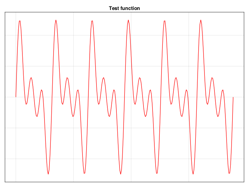
This machinery allows testing all the different implementations in a reproducible way. All the examples given in this article are calculated on the following input signal.
Using arduino-cli to upload your code.
At the time I started this project, the new Arduino IDE wasn't available yet. If you have ever used the 1.x versions of the IDE, then you know why one would like to avoid the old IDE. Thankfully, there is a command-line utility that allows uploading code from your terminal: arduino-cli. If you take a look at the GitHub repository, you'll notice a Julia script, which purpose is to upload code to the Arduino and retrieve the results of computations and benchmarks. The upload part is simply a system call to arduino-cli.
function upload_code(directory)
    build = joinpath(workdir, directory, "build")
    ino = joinpath(workdir, directory, directory * ".ino")

    build_command = `arduino-cli compile -b arduino:avr:uno -p $portname --build-path "$build" -u -v "$ino"`
    run(pipeline(build_command, stdout="log_arduino-cli.txt", stderr="log_arduino-cli.txt"))
end
Don't bother with communication protocols over Serial.
At first, I was tempted to use some fancy communication protocols for the serial link. This is not useful in our case, because you can simply reset the Arduino programmatically to ensure the synchronization of the computer and the development board, and then exchange raw binary data.
Resetting is done using the DTR pin of the port. In Julia, you can do this like this using the LibSerialPort.jl library:
function reset_arduino()
    LibSerialPort.open(portname, baudrate) do sp
        @info "Resetting Arduino"
        # Reset the Arduino
        set_flow_control(sp, dtr=SP_DTR_ON)
        sleep(0.1)
        set_flow_control(sp, dtr=SP_DTR_OFF)
        sp_flush(sp, SP_BUF_INPUT)
        sp_flush(sp, SP_BUF_OUTPUT)
    end
end
Because your computer can now reset the Arduino at will, you can easily ensure the synchronization of your board. That means the benchmark script knows when to read data from the Arduino.
Then, the Arduino would send data to the computer like this:
Serial.write((byte*)data, sizeof(fixed_t)*N);This way, the array data is sent directly through the serial link as a stream of raw bytes. We don't bother with any form of encoding.
On the computer side, you can easily read the incoming data:
data = zeros(retrieve_datatype, n_read)
read!(sp, data)
Where sp is an object created by LibSerialPort.jl when opening a port.
You can then happily analyze your data, it's DataFrames.jl and Makie.jl time !
Fast, accurate FFT, and other floating-point trickeries.
My first approach was to re-use as much as I could the code I wrote for my FFT tutorial in Julia. That's why I started working with floating-point arithmetic. This also was convenient because it kept away some issues like overflowing numbers, that I had to address once I started working with fixed-point arithmetic.
A first dummy implementation of the FFT.
As I said, my first implementation was a simple, stupid translation of one of the codes presented in my Julia tutorial. I did not even bother with writing optimized trigonometry functions, I just wanted something that worked as a basis for other implementations. The code is fairly simple and can be viewed here.
As expected, this gives almost error-free results.

Forbidden occult arts are fun. 😈
Now let's move on to more interesting stuffs. The first obvious improvement you can make on the base implementation is fast trigonometry, and that's what yields the biggest improvement in terms of speed. Then, I decided to mess around with IEEE-754 to write my own approximate routines for float multiplication, halving and modulus calculation. The idea is always the same: treat IEEE-754 representation of a floating-point number as its logarithm. This does give weird-looking implementations though. I have written several posts on Zeste-de-Savoir explaining how all these work. It is in French, but I trust you can make DeepL run!
"Approximer rapidement le carré d'un nombre flottant" explains how to square a number using its floating-point representation.
"IEEE 754: Quand votre code prend la float" explains how the IEEE-754 representation of a number looks alike it's logarithm.
"Multiplications avec Arduino: jetons-nous à la float" explains how the approximate multiplication of two floating-point numbers can be efficiently calculated.
Approximate floating-point FFT.
Without further delay, here is a sneak preview of the result I got with the approximate floating-point FFT. For a full benchmark, you will have to wait for the end of this article! The code is available here.

How fixed-point arithmetic came to the rescue.
Rather than endlessly optimizing the floating-point implementation, I decided to change my approach. The main motivation being: Floats are actually overkill for our purpose. Indeed, they have the ability to represent numbers with a good relative precision over enormous ranges. However, when calculating FFTs the range output variables may cover can indeed vary, but not that much. And most importantly, it varies predictably. This means a fixed-point representation can be used. Also, because of their amazing properties Floats actually take a lot of space in the limited RAM available on a microcontroller. And finally, I want to be able to run FFTs on signal read from Arduino's ADC. If my program can deal with int-like data types, then it'll spare me the trouble of converting from integers to floating-points.
Fixed-point multiplication.
I first played with the idea of implementing a fixed-point FFT because I realized the AVR instruction set gives us the fmul instruction, dedicated to multiplying fixed-point numbers. This means we can use it to have a speed-efficient implementation of the multiplication, that should even beat the custom float one.
I wrote a blog-post on Zeste-de-Savoir (in French) on implementing the fixed-point multiplication. It is based on the proposed implementation in the AVR instruction set manual.
/* Signed fractional multiply of two 16-bit numbers with 32-bit result. */
fixed_t fixed_mul(fixed_t a, fixed_t b) {
  fixed_t result;
  asm (
      // We need a register that's always zero
      "clr r2" "\n\t"
      "fmuls %B[a],%B[b]" "\n\t" // Multiply the MSBs
      "movw %A[result],__tmp_reg__" "\n\t" // Save the result
      "fmul %A[a],%A[b]" "\n\t" // Multiply the LSBs
      "adc %A[result],r2" "\n\t" // Do not forget the carry
      "movw r18,__tmp_reg__" "\n\t" // The result of the LSBs multipliplication is stored in temporary registers
      "fmulsu %B[a],%A[b]" "\n\t" // First crossed product
                                  // This will be reported onto the MSBs of the temporary registers and the LSBs
                                  // of the result registers. So the carry goes to the result's MSB.
      "sbc %B[result],r2" "\n\t"
      // Now we sum the cross product
      "add r19,__tmp_reg__" "\n\t"
      "adc %A[result],__zero_reg__" "\n\t"
      "adc %B[result],r2" "\n\t"
      "fmulsu %B[b],%A[a]" "\n\t" // Second cross product, same as first.
      "sbc %B[result],r2" "\n\t"
      "add r19,__tmp_reg__" "\n\t"
      "adc %A[result],__zero_reg__" "\n\t"
      "adc %B[result],r2" "\n\t"
      "clr __zero_reg__" "\n\t"
      :
      [result]"+r"(result):
      [a]"a"(a),[b]"a"(b):
      "r2","r18","r19"
  );
  return result;
}
Obviously, you can also create the same function for 8-bits fixed-point arithmetic.
fixed8_t fixed_mul_8_8(fixed8_t a, fixed8_t b) {
  fixed8_t result;

  asm (
    "fmuls %[a],%[b]" "\n\t"
    "mov %[result],__zero_reg__" "\n\t"
    "clr __zero_reg__" "\n\t"
    :
    [result]"+r"(result):
    [a]"a"(a),[b]"a"(b)
  );
  return result;
}
As you can see, this requires writing some assembly code because the fmul instruction is not directly accessible from C. However, even though it is fairly simple, this limits the implementation to AVR platforms. You might still get some reasonably efficient code by implementing everything in pure C, and extend the implementation to other platforms.
Controlled result growth.
As I said before, the FFT grows predictably. First, we can see that the final Fourier transform is bounded. Recall that the FFT is an algorithm to compute the Discrete Fourier Transform (DFT), which is written:
\[\begin{aligned} X[k] &=& \sum_{n=0}^{N-1}x[n]e^{-2i\pi nk/N} \end{aligned}\]Where \(X\) is the discrete Fourier transform of the input signal \(x\) of size \(N\). From that we have:
\[\begin{aligned} |X[k]| &\leq \left|\sum_{n=0}^{N-1}x[n]e^{-2i\pi nk/N}\right|\\ &\leq \sum_{n=0}^{N-1}\left|x[n]e^{-2i\pi nk/N}\right| \\ &\leq \sum_{n=0}^{N-1}\left|x[n]\right|\\ &\leq N\times\max_n|x[n]| \end{aligned}\]In our case, because we use the Q0f7 fixed point format, the input signal \(x\) is in the range \([-1,1]\). That means the components of the DFT are within range \([-N,N]\). Note that these bounds are attained for some signals, e.g. a constant input.
With that, we know how to scale the result of the FFT so that it can be stored. But what about the intermediary steps ? How do we ensure that the intermediary values stay within range? You may recall from the blog post explaining FFT this kind of "butterfly" diagrams:
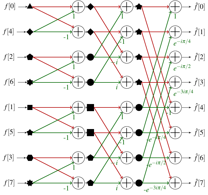
This diagram also shows you that each step of the algorithm actually performs some FFTs on input signals of smaller sizes. That means our bounding rule applies for intermediary signals, given that we plug the right size of input signal in the formula! Notice how at each step, corresponding sub-FFTs have a size of \(2^{i}\), where \(i\) is the number of the step, starting at 0. That basically means that if we scale down the signal between each step by dividing it by a factor of two, we will keep the signal bounded in \([-1,1]\) at each step!
Note that this does not mean we get the optimal scale for every input signal. For example, signals which are poorly periodic would have a lot of low module Fourier coefficients, and would not fully take advantage of the scale offered by our representation. I did some tests scaling the array only when it was needed, and did not notice many changes in terms of execution times, so that's something you might want to explore if your project requires it.
Trigonometry is demanding.
If all you have is a hammer, everything looks like a nail.
Once I had fixed-point arithmetic working, I started wanting to use it everywhere. But I quickly encountered an issue: trigonometry stopped working.
The reason is simple, 8-bits precision is not enough for trigonometry calculations when we approach the small angles. The key point here, is that the precision needed for fixed-point calculation of trigonometry functions depends on the size of the input array. Recall from section Trigonometry can be blazingly fast. 🚀🚀🚀 🔥🔥 that we need to precompute values for \(\alpha\) and \(\beta\), where
\[\alpha = 2\sin^2\left(\frac{\delta}{2}\right),\quad\beta=\sin\delta\]And \(\delta\) is the angle increment by which we want to increase the angle of the complex number we are summing with in the FFT. This angle depends on \(N\), the total length of the input array, and is equal to \(\frac{2\pi}{N}\). That means we need to be able to represent at least \(2\sin^2\frac{\pi}{N}\) for trigonometry to work. For \(N=256\), this is approximately equal to \(0.000301\). Unfortunately, the lowest number one can represent using Q0f7 fixed point representation, that is with 7 bits in the fractional part, is \(2^{-7}=0.0078125\). That is why even for the 8 bit fixed point FFT, trigonometry calculations are performed using 16 bits fixed point arithmetic.
This limit on trigonometry also explains why the code presented here is not usable "as is" for very long arrays. Indeed, while 512 cases-long arrays could be handled using 16-bits trigonometry, the theoretical limit for an Arduino Uno would be 1024 cases-long arrays (because RAM is 2048 bytes, and we need some space for temporary variables), and that would require 32-bits trigonometry, which I did not implement.
Saturating additions. (a.k.a. "Trigonometry is demanding" returns.)
One other issue with trigonometry I did not see coming is its sensitivity to overflow. Since there is basically no protection against it, overflowing a fixed-point representation of a number flips the sign. In the case of trigonometry this is especially annoying, because that means we add a \(\pi\) phase error for even the slightest error when values are close to one. And trust me, it took me some time to understand where the error was coming from.
To mitigate this, I had to implement my own addition, that saturates to one instead of flipping the sign when overflow happens. The trick here is to use the status register (SREG) of the microcontroller to detect overflow. Again this requires doing the addition in assembly, as the check needs to happen right after the addition was performed, and there is no way to tell what the compiler might do between the addition and the actual check.
Checking overflow is done using the brvc instruction (Branch if Overflow Cleared), and the function for 16-bits saturating addition goes like this:
/* Fixed point addition with saturation to ±1. */
fixed_t fixed_add_saturate(fixed_t a, fixed_t b) {
  fixed_t result;
  asm (
      "movw %A[result], %A[a]" "\n\t"
      "add %A[result],%A[b]" "\n\t"
      "adc %B[result],%B[b]" "\n\t"
      "brvc fixed_add_saturate_goodbye" "\n\t"
      "subi %B[result], 0" "\n\t"
      "brmi fixed_add_saturate_plus_one" "\n\t"
      "fixed_add_saturate_minus_one:" "\n\t"
      "ldi %B[result],0x80" "\n\t"
      "ldi %A[result],0x00" "\n\t"
      "jmp fixed_add_saturate_goodbye" "\n\t"
      "fixed_add_saturate_plus_one:" "\n\t"
      "ldi %B[result],0x7f" "\n\t"
      "ldi %A[result],0xff" "\n\t"
      "fixed_add_saturate_goodbye:" "\n\t"
      :
      [result]"+d"(result):
      [a]"r"(a),[b]"r"(b)
  );

  return result;
}
One might be tempted to use this routine for every single addition performed in the program. This is actually useless, since additions in the actual FFT algorithm will not overflow thanks to scaling, if they are done in a sensible order (check the code if you want to see how!).
Calculating modules with a chainsaw.
After a lot of wandering on the Internets, I ended up using Paul Hsieh's technique for computing approximate modules of vectors. However, while writing this article I discovered some mistakes and things that could be improved in his article, so I ended up writing a dedicated article on this, showing how you can minimize the mean square error, and get at most a 5.3% error.
The main idea is that you can approximate the unit circle using a set of well-chosen octagons. That reminds me of what a rough cylinder carved using a chainsaw might look like, hence the name of this section.

16 bits fixed-point FFT.
Enough small talk, time for some action! You can find here the code for 16-bits fixed-point FFT. The benchmark is available at the end of this article, but in the meantime here is the error comparison against reference implementation.

8 bits fixed-point FFT.
And now the fastest FFT on Arduino that I implemented, the 8-bits fixed-point FFT! As for previous implementations, you can find the code here. Below is a comparison of the calculated module of the FFT against a reference implementation.

Implementing fixed-point FFT for longer inputs
The Arduino Uno has 2048 bytes of RAM. But because this implementation of the FFT needs an input array whose length is a power of two, and because you need some space for variables,[3] the limit would be a 1024 bytes long FFT. But the code presented here would have to be modified a bit (not that much). From where I am standing I see two major issues:
As discussed previously, trigonometry would need 32-bits arithmetic. That means you would need to implement the multiplication and saturating addition for those numbers.
The buffers are single bytes right now, so you would need to upgrade them to 16-bits buffers.
Once those two issues, and the inevitable hundreds of other issues I did not think of are addressed, I don't see why one could not perform FFT on 1024 bytes-long input arrays.
| [3] | Although I am sure a very determined person would be able to fit all the temporary variables in registers and calculate a 2048 bytes-long FFT. Do it, I vouch for you, you beautiful nerd! |
Benchmarking all these solutions.
I won't go into the details of how I do the benchmarks here, it's basically just using the Arduino micros() function. I present here only two benchmarks: how much time is required to run the FFT, and how "bad" the result is, measured with the mean squared error. Now, this is not the perfect way to measure the error made by the algorithm, so I do encourage you to have a look at the different comparison plots above. You will also notice that ApproxFFT seems to perform poorly in terms of error for small-sized input arrays. This is because it does not compute the result for frequency 0, so the error is probably over-estimated. Overall, I think it is safe to say that ApproxFFT and Fixed16FFT introduce the same amount of errors in the calculation. Notice how ExactFFT is literally billions times more precise than the other FFT algorithms. For 8-bits algorithms, the quantization mean squared error is \({}^1/{}_3 LSB^2\approx2\times10^{-5}\), which means there are still sources of error introduced in the algorithm other than simple quantization. The same goes for ApproxFFT and Fixed16FFT, where the quantization error is approximately \(3\times10^{-10}\).

Execution time is where my implementations truly shine. Indeed, you can see that for 256 bytes-long input array, Fixed8FFT only needs about 12 ms to compute the FFT, when it takes 52ms for ApproxFFT to do the same. And if you need the same level of precision as what ApproxFFT offers, you can use Fixed16FFT, which only needs about 30ms to perform the computation. It's worth noticing that FloatFFT is not far behind, with only 67ms needed to compute the 256 bytes FFT. Of course Exact FFT takes much longer.

Closing thoughts.
It has been a fun journey! I had a lot of fun and "ha-ha!" moments when debugging all these implementations. As I wrote before, there are ways to improve them, either by making Fixed8FFT able to handle longer input arrays, or writing a custom-made addition for floating-point number to speed-up FloatFFT. I don't know if I will do it in the near future, as this whole project was just intended to be a small side-project, which ended-up bigger than expected.
As always, feel free to contact me if you need any further detail on this. You can join me on mastodon, or on GitHub, or even through the comment section below! In the meantime, have fun with your projects. :)